Learn how to sum up checkboxes in Google Sheets
Learn how to sum up Checkboxes in Google Sheets in to a separate column to create summaries and aggregate data for analysis.
Introduction
Google Sheets allows you to change a column data type to checkboxes for easier data entry. However, it poses a few challenges if you’re trying to use this data for further analysis in Google Sheets like when you try to sum up checkboxes in Google Sheets.
Why is it difficult to work with checkboxes in Google Sheets?
The reason is simple: not many people know how this data is stored in the backend. Also, changing the formatting of these columns removes the checkboxes from the view. Although it makes it easier to enter data, it is not easy to model further analysis of these data columns that have checkboxes.
Learn how to automatically apply formulas to new rows in Google Sheets.
Glide provides easier ways to do accomplish tasks like summing up checkboxes in Google Sheets.
Sample data to learn how to sum up checkboxes in Google Sheets
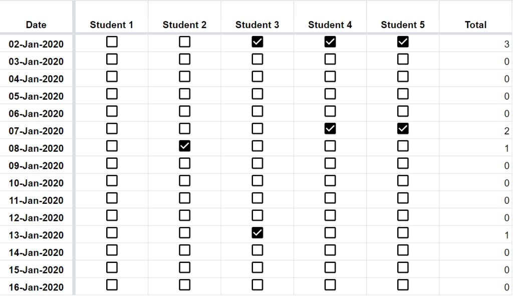
The following version of a Google Sheets document illustrates this problem: a simple attendance management system. Column A has dates, while columns B to F have names of students. Attendance is marked using checkboxes in columns B to F.

The challenge here is to find the number of students who attended the class on any given day. The last column – ‘Total’ – indicates the total number of students who attended the class on that particular day.
Without understanding how the data is stored behind a cell with a checkbox, it is difficult to create any formulas to give us the answer.
Formula to sum up checkboxes in Google Sheets
Checkboxes are stored as boolean values (TRUE or FALSE) in Google Sheets.
So the trick is to treat these cells as if they contain TRUE or FALSE values and then model the analysis accordingly.
In this case, imagine columns B to F to have an array of TRUE and FALSE values. You can then use this array as one input in the SUMPRODUCT formula and use an array of 1s as the second input. The number of 1s in the second input will be the same as the number of students – in this case, 5.
=SUMPRODUCT(B2:F2,{1,1,1,1,1})