How to highlight duplicates in Google Sheets

Introduction

Time and again you will find yourself in the middle of messy data and wondering, among many other data cleanup activities, how to highlight duplicates in Google Sheets.

Conditional formatting, although computation intensive if the database size is enormous, allows you to identify duplicates proactively, instead of trying to find duplicates in Google Sheets manually every time.

Structure of the Sample Google Sheet

The live Google Sheets workbook for this exercise is posted here and is split across 4 tabs as of today:

1. Data: Input data for this exercise.
2. Highlighting Cell in a Column: How to highlight duplicate cells in a column?
3. Highlighting Entire Row: How to highlight an entire row based on a duplicate value in a column?
4. Highlighting Subsequent Duplicate Rows: How to highlight only subsequent duplicate rows based on an identical value in a column?

In the sample data, no two different customers can have the same Customer ID, and therefore the challenge here is to identify:

1. All duplicate entries for the same customer.
2. Ensure that the same Customer ID is not assigned to two different customers.

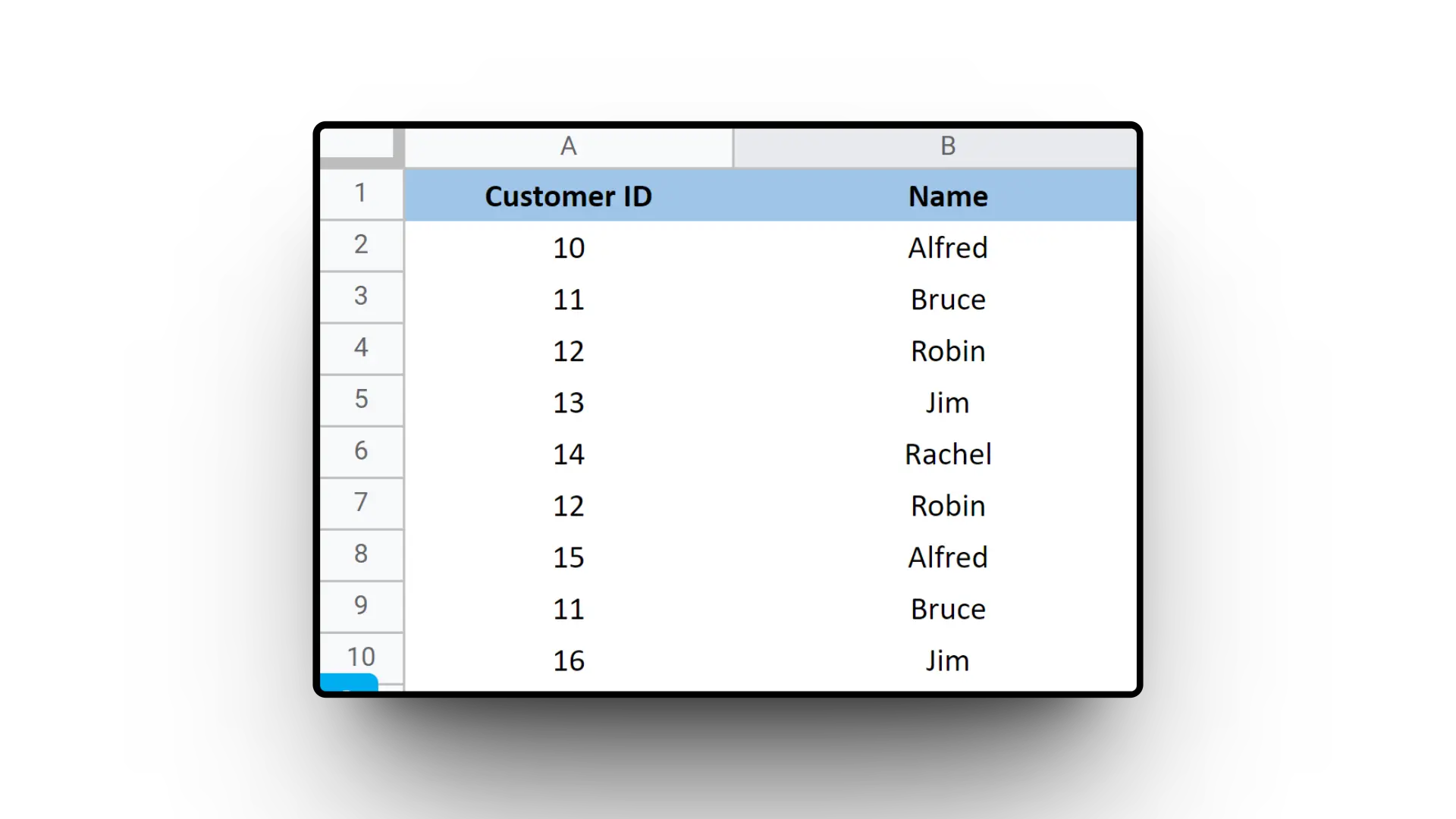
How to find Conditional Formatting options in Google Sheets

There are two ways to find the Conditional Formatting menu:

1. Main Menu –> Format –> Conditional Formatting
2. Right-click a cell –> Conditional Formatting

Find a cell with duplicate contents in a column

Switch to tab: Highlighting Cell in a Column in the workbook to understand the output of this exercise.

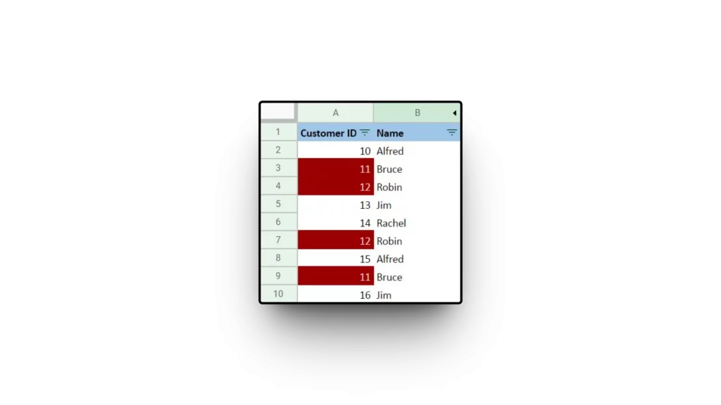
The idea here is to highlight only one value based on the column of interest.

1. Open the Conditional Formatting Menu.
2. Enter A2:A in the Apply to range input area. Google Sheets will automatically update the range to indicate the maximum number of rows in the sheet.
3. Under the Format rules section, from the dropdown menu, select ‘Custom formula is‘.
4. In the area provided, enter the formula =COUNTIFS($A$2:$A,$A2)>1.
5. This formula evaluates if there are more than one instance of the value in cell A2 in the range A2:A.
6. Conditional formatting always applies when the result of the formula/condition is TRUE.
7. When done, all the cells in column A with duplicate entries will be highlighted using the formatting chosen in the Conditional formatting menu, in this case, magenta background color with light pink text color.

Highlighting the entire row with duplicate contents

Switch to tab: Highlighting Entire Row in the workbook to understand the output of this exercise.

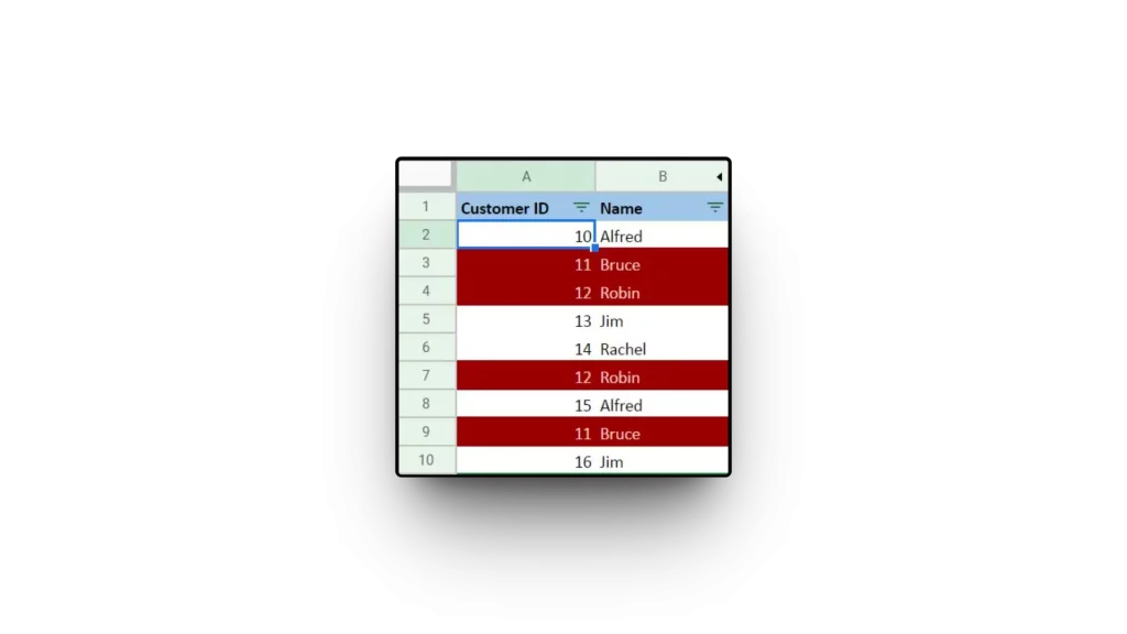
The idea here is to highlight the entire row based on the value in the column of interest.

• Repeat everything listed in the solution to Challenge 1, except for one change: the range.
• Enter A2:B in the Apply to range input area. Google Sheets will automatically update the range to indicate the maximum number of rows in the sheet.

Highlighting subsequent duplicate rows

Switch to tab: Highlighting Subsequent Duplicate Rows in the workbook to understand the output of this exercise.

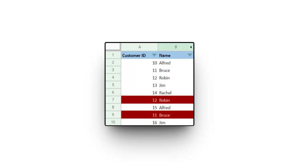
The idea here is to highlight the entire row based on the value in the column of interest, except for the first occurrence of the duplicate row.

• Repeat everything listed in the solution to Challenge 1, except for two changes: the range, and the formula.
• Enter A2:B in the Apply to range input area. Google Sheets will automatically update the range to indicate the maximum number of rows in the sheet.
• Under the Format rules section, from the dropdown menu, select Custom formula is. In the area provided, enter the formula =COUNTIFS($A$2:$A2,$A2)>1. Instead of looking in the entire column, we are looking for duplicates only up to the row in question. So, to check if the Customer ID in row 4 has already been entered into the list, we will check all rows from Row 2 to Row 4, and not in all the rows.

Summary

Using conditional formatting, you can highlight duplicate cells in a column and an entire row based on the value in a specific column. You can also highlight only subsequent identical values after the first occurrence.